
HOUDINI TORNADO (HIP FILE INCLUDED)
This is a Technical Breakdown of my Houdini FX Tornado.
Here is the HIP file for the corresponding technical breakdown, from setup to customization options. PLEASE don’t just copy and paste my work, learn from it and make it better. We are artists after all. You might just find a better, more efficient technique!
HIP File:
https://drive.google.com/file/d/1nzeu2Z5GT6Xu2HDLZVU3ASJ2t81Xe_mf/view?usp=sharing
For my Full Process of building this from start to finish, view my blog page here:
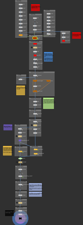
For the quick and easy spark notes, here is a concise HIP file breakdown and my personal technical process:
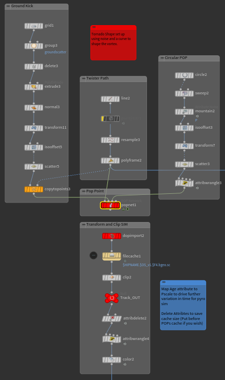
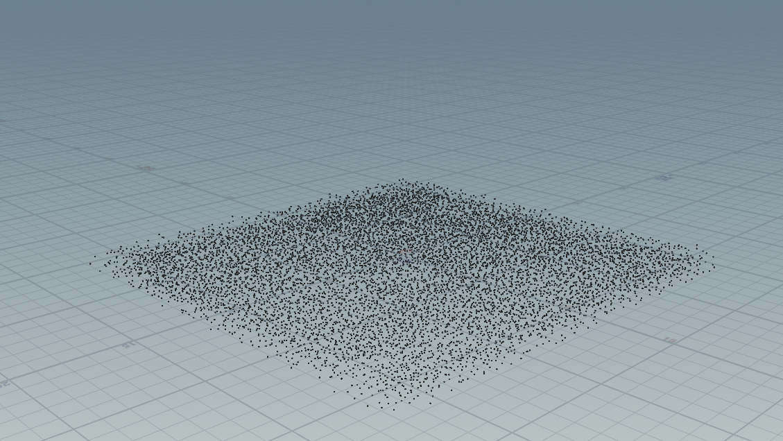
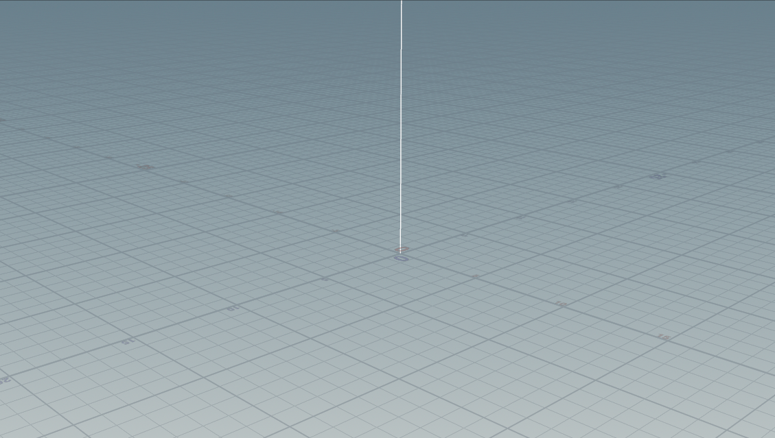
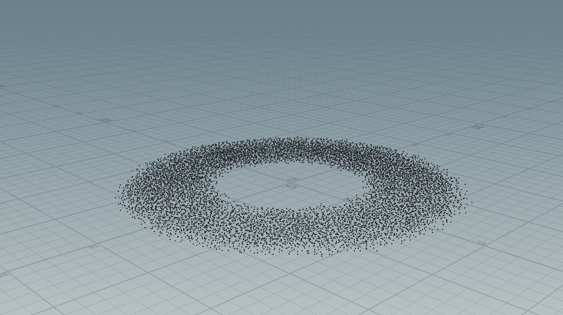
To begin building the tornado, I start with a few different pieces of geometry and scatter points inside them to generate the birth locations for the POP simulation. In this case, I use a swept circle combined with an animated Mountain node to introduce additional variation and motion. I also create a simple line that defines the main tangent the vortex will follow. For this demonstration, the line remains un-jittered, but you can freely bend or distort it to shape the vortex path however you like.
Below is a visual of the primary setup, followed by a breakdown of the POP network.
You can then take your scattered points and tangent line into POPs, where the real simulation and actual vortex creation begins.
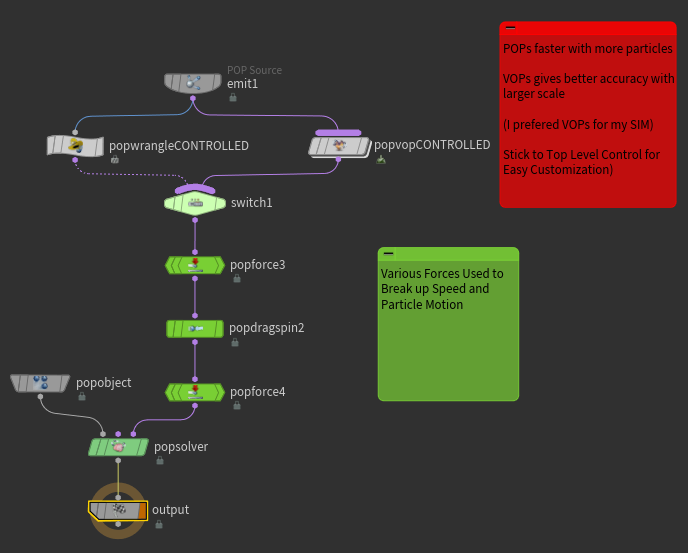
Both the VOP and VEX approaches achieve the exact same result, just through different workflows. The vortex was originally built using VOPs, but I recreated it in VEX to gain a better understanding of working with point clouds. While VOPs felt more intuitive and easier to organize, I found that VEX performed noticeably faster when it came to caching. This particular setup caches relatively quickly, but the performance difference becomes more important in heavier simulations, such as those with complex collisions or high substeps.
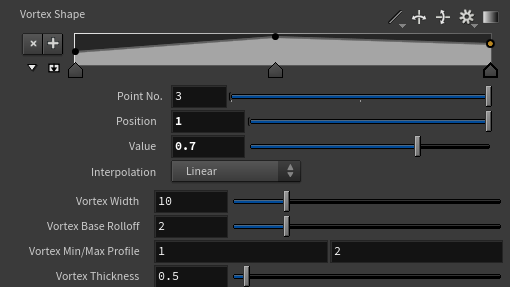
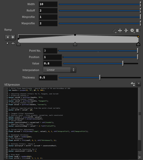
Both approaches expose top-level parameters that allow you to control the vortex’s width, width falloff, profile size, and overall thickness. The overall shape can also be further refined using the ramp controls. Feel free to adjust these parameters to suit your specific use case.
Below is a detailed explanation of the code and how it works.
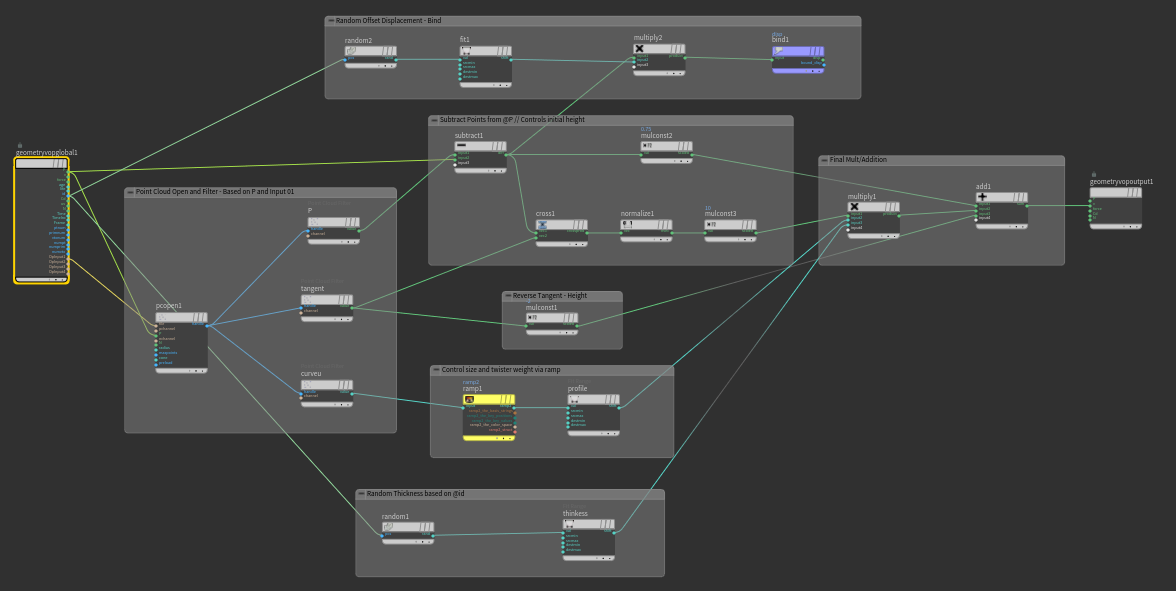
VEX & VOPs Breakdown
This setup samples nearby points, extracting directional data, and combining multiple forces into a final velocity field. Both the VEX and VOP approaches achieve the same result, the difference is purely workflow and visualization.
At its core, this system:
Samples nearby points (point cloud)
Extracts averaged attributes (position, tangent, curve position)
Builds directional and rotational forces
Layers in artistic controls (ramps, randomness)
Outputs a final swirling velocity (@v)
1 - Point Cloud Sampling
VEX: pcopen + pcfilter
VOPs: Point Cloud Open + Point Cloud Filter
Finds neighboring points within a radius
Averages attributes like:
P (position)
tangent (flow direction)
curveu (position along curve)
2 - Base Direction (Attraction)
VEX: diffP = valueP - @P
VOPs: Subtract node
Computes direction toward the averaged position
Acts as a stabilizing force, keeping particles bound to the vortex shape
3 - Rotational Force (Swirl)
VEX: cross(diffP, tangent) → normalize
VOPs: Cross Product → Normalize → Multiply
Cross product generates a perpendicular vector
This creates circular motion around the flow
Scaled to control vortex width and intensity
This is the “spin” of the tornado.
4 - Opposing Constraint (Balance)
VEX: negative tangent contribution
VOPs: Multiply tangent by negative value
Adds a counterforce to prevent unstable motion
Helps maintain a cohesive vortex structure
5 - Height/Profile Control
VEX: chramp("ramp", curveU)
VOPs: Ramp Parameter
Shapes the vortex along its height
Controls where the effect is stronger or weaker
Used to modulate twist, width, or influence
6 - Thickness & Variation
VEX: random(@id) + fit()
VOPs: Random → Fit Range
Adds per-point variation
Breaks uniform motion
Controls thickness and density of the vortex
7 - Offset / Displacement
VEX: additional random scaling of diffP
VOPs: Random → Fit → Multiply
Introduces subtle positional offsets
Helps avoid overly clean or rigid motion
8 - Combining Forces
VEX: sum of all vectors
VOPs: Multiply + Add chain
Base attraction (diffP)
Rotational force (cross product)
Profile shaping (ramp)
Thickness variation
Counterforce (negative tangent)
All influences are layered together into a single velocity vector.
9 - Final Output
VEX: @v = twist;
VOPs: Bind Export (v)
The final vector drives particle motion
Produces a stable, art-directable vortex effect
Key Differences:
VEX
Faster to evaluate and cache
More compact and flexible
Better for optimization and scaling
VOPs
Visual and easier to debug
Clear node-based flow
Great for understanding relationships between forces
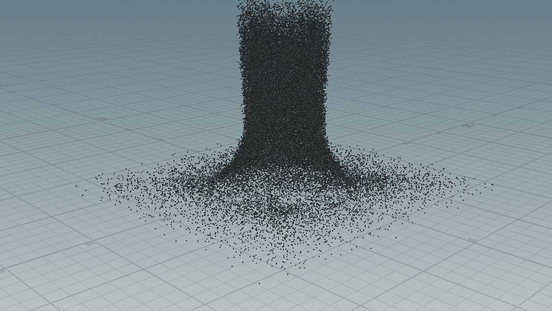
Whether you choose the Wrangle or VOP-based approach, you should arrive at a similar result, as shown below. The motion should resemble that of a vortex, with size, width, and thickness driven by the parameters you’ve set. If your simulation doesn’t match the reference, double-check that no nodes are disabled in your VOP network or that no lines have been accidentally removed from your Wrangle, either can easily break the setup.
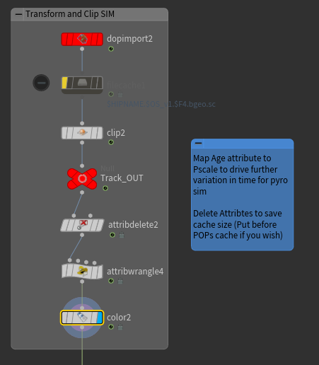
After simulating your POPs, you can optionally clean up by removing unnecessary attributes and driving pscale based on the age of the particles. This can help add more detail in later stages. I applied this technique in my final render, as it better matched the look I was aiming for.
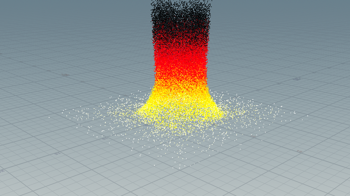
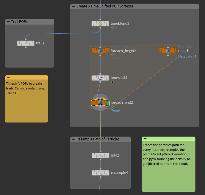
With the simplified POPs in place, you can add a Trail SOP or achieve a similar result with more control by using Time Shift, as shown below. Introducing a bit of echo to the POPs can also help generate more interesting motion, which will better drive the simulation in later stages.
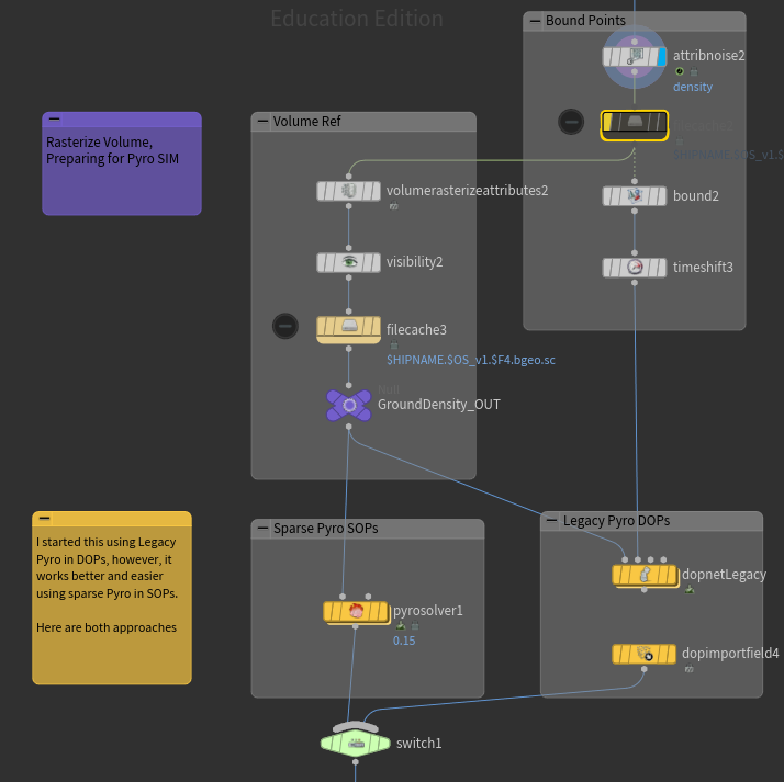
Using the Pop Trail, the attributes are now ready to be rasterized and fed into the simulation. In my file, I’ve set up two different approaches, each with distinct use cases and reasons for choosing one over the other. I’ve traditionally been a “do it in DOPs” artist and still tend to lean that way, especially for RBD work, because it offers maximum control over every aspect of the simulation, with parameters set up manually. This level of control can add stability to otherwise complex setups.
That said, the SOP-level Pyro Solver is extremely stable and reliable, making it a great choice for simpler effects. Since this particular simulation is fairly straightforward, it doesn’t require anything overly complex. SOP-level DOPs are especially useful for quick, efficient setups, and I often use them in those scenarios. Below is the layout showing the flow from SOPs into DOPs for simulating the vortex.
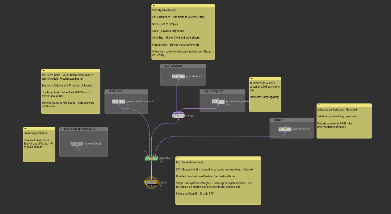
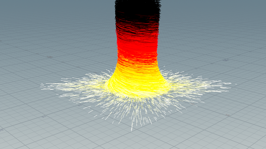
Using the exact parameters from above, I created a quick playblast to show the full simulation in its default state. While it’s not yet a picture-perfect tornado, achieving that would require further parameter adjustments, it serves as a solid foundation. Think of it as a large block of stone that you can gradually refine by adding detail such as turbulence, disturbance, and shredding. You can also revisit earlier stages of the setup, like Pop Force or Pop Drag, to introduce more variation and break up the motion.
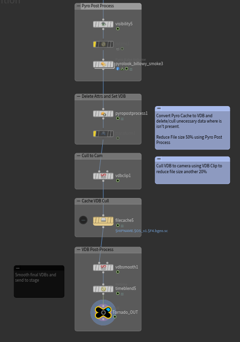
The final touches for this simulation involve baking the volume and converting it to VDB/16-bit float to reduce cache size. I also focus on culling geometry and simulations to the camera’s view; a simple VDB Clip node makes this process straightforward. After caching, I sometimes apply a subtle smoothing pass to eliminate any hard edges in the simulation, though this step is entirely optional depending on the desired look.
I hope this HIP file and breakdown helps in whatever way you found yourself needing it! Feel free to message me via email or LinkedIn should you find any more efficient method for this type of FX. Cheers!